Optimization in Mechanical Engineering

Description

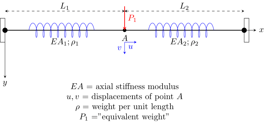
Using the optimization methods implemented in optymus: (a) determine the displacements \((u, v)\), of point A, that minimize the Total Potential Energy (\(\Pi\)) of the spring system indicated in the figure below. Adopt the following numerical values:

• Initial points: \(x0 = \{15, 12\}^t\) e \(x0 = \{9, −2\}^t\);

• \(L1 = 12 cm\);

• \(L2 = 8\) cm;

• \(EA1 = 12 N\) ;

• \(EA2 = 80 N\) ;

• \(\rho 1 = 0.82 N/cm\);

• \(\rho 2 = 0.52 N/cm\);

We can see the system in the image below:

We can optimize the system by minimizing the total potential energy of the system, which is given by:

\[\Pi = \frac{1}{2} \left( EA1 \cdot \rho1 \cdot (L1 - \sqrt{u^2 + v^2})^2 + EA2 \cdot \rho2 \cdot (L2 - \sqrt{u^2 + v^2})^2 \right)\]

and numerically,

\[\Pi = 5(((x_1 - 8)^2 + x_2^2)^{1/2} - 8)^2 - 7x_2 + 0.5(((x_1 + 12)^2 + x_2^2)^{1/2} - 12)^2\]

Implementation

from optymus import Optimizer

import jax.numpy as jnp

def f(x):
    return 5 * (((x[0] - 8)**2 + x[1]**2)**0.5 - 8)**2 - 7 * x[1] + 0.5 * (((x[0] + 12)**2 + x[1]**2)**0.5 - 12)**2

initial_point = jnp.array([9.0, -2.0])

opt = Optimizer(f_obj=f, x0=initial_point, method='steepest_descent')

Steepest Descent 0:  34%|███▍      | 34/100 [00:02<00:04, 15.15it/s]

opt.report()

[-] steepest_descent

Initial guess: [ 9. -2.]

Optimal solution: [2.78529691 6.89972057]

Objective function value: -36.880428392231394

Number of iterations: 34

Time elapsed: 2.5588

opt.plot(lb=-25, ub=25, n_levels=150)